Monte Carlo Integrals over $\mathbb{R}$

Monte Carlo integration provides a way to compute integrals numerically with an algorithm that has the same convergence class (uncertainty $\sim \mathcal{O}(1/\sqrt{N})$ ) independently of the dimension of the integration domain (as opposed to methods like the trapezoid approximation).

Integrating over a finite volume is quite easy: you need to find a parametrization of your domain such that each variable spans a fixed interval and one can then rely on any strictly probability distribution over this interval to sample points.

$$\int_{a}^{b} dx f(x) = \int_{a}^{b} dx p(x) \dfrac{f(x)}{p(x)} = \underset{x\sim p}{\mathbb{E}} \dfrac{f(x)}{p(x)}$$

In particular, if one samples uniformly,

$$\int_a^b dx f(x) = (b-a) \times\underset{x\sim U_{[a,b]}}{\mathbb{E}}f(x)$$

Sampling over all of $\mathbb{R}$ is, however, slightly more complicated. The first idea one could have would be to observe that any function we integrate should go to zero fast enough at infinity. As a result, it seems reasonable to integrate over a finite, large enough interval, and maybe even try to extrapolate the result from multiple interval sizes.

The issue with this approach is that, while it is always possible to evaluate an integral over such a finite volume, the variance of the result will reach infinity as we grow the interval size. Meaning that there is a conflict between needing to increase the interval size to get a good approximation of the infinite integral and having ever less accurate estimates.

It is quite easy to show how this problem arises:

Let us integrate a function over an interval of size $L$, symmetric around 0

$$I(L) = \int_{-L/2}^{L/2} dx f(x) = L \times\underset{x\sim U_{L}}{\mathbb{E}}f(x)$$

If we build a flat Monte Carlo estimator, $\hat{I}(L) = L f(X), X\sim U_L$ , we can easily compute its variance:

$$\sigma^2\left(\hat{I}(L)\right) = L^2 \left(\underset{x\sim U_{L}}{\mathbb{E}}\left(f(x)^2\right) - \left(\underset{x\sim U_{L}}{\mathbb{E}}f(x)\right)^2\right) = L \int_{-L/2}^{L/2} dx f(x)^2 - I(L)^2$$

The variance is finite if $f^2$ is integrable. However, it grows linearly with the size of the integral. Depending on the functio n to integrate, this might or might not be a problem, as illustrated below, but in general, the method is unreliable and not guaranteed to work.

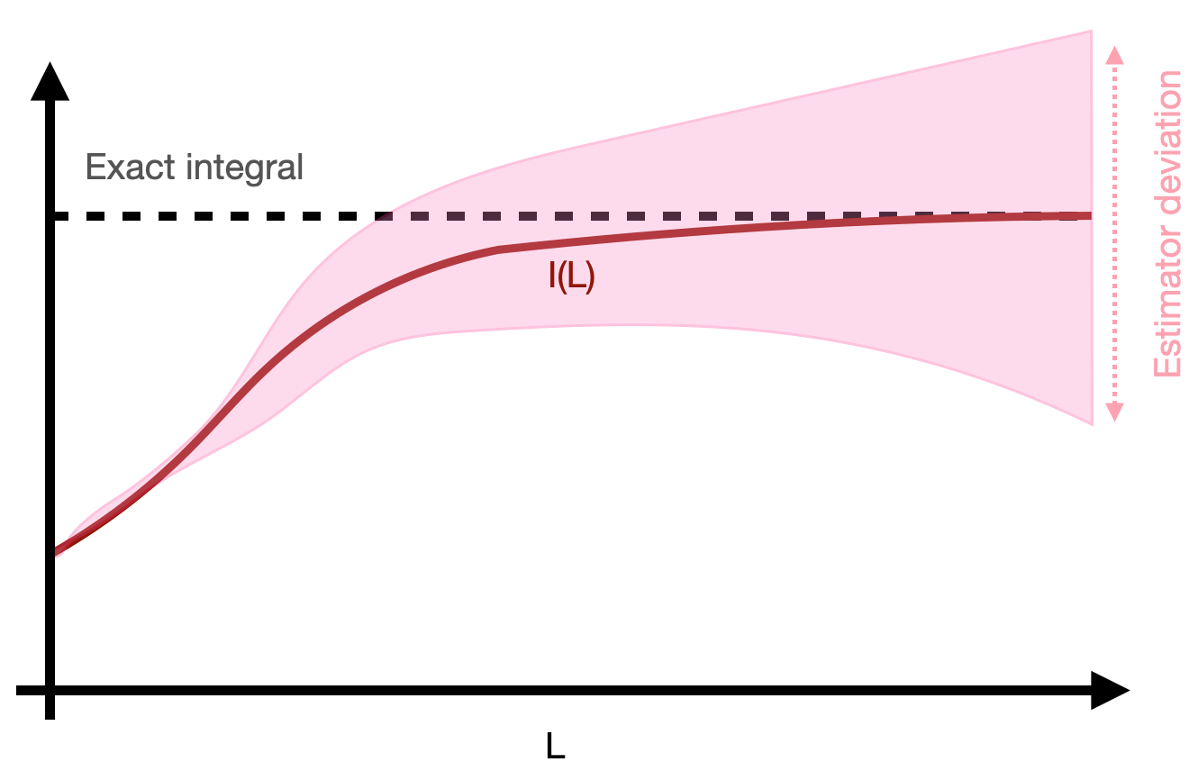If the variance of the estimator grows too fast before the finite-volume integral approximates the full integral well, we cannot use uniform sampling.

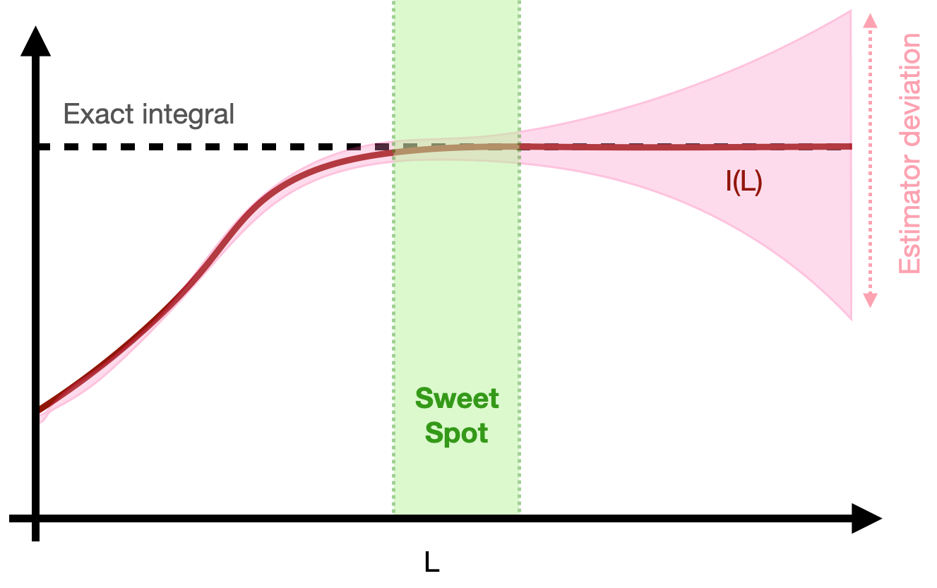If the finite-volume integral converges to the full integral faster than the variance diverges, there might be a sweet spot where we have a good approximation with a manageable variance.

An astute observer would determine that the low-level mechanistic reason why we are having this issue is that we are using a uniform sampling procedure, which makes this annoying factor of $L$ appear in front of the variance. A more high-minded way of saying this is that we keep thinning out the amount of sampling that we do in the regions where $f$ has a significant contribution as we expand the integration region, which in turns increases the variance in an unsustainable way.

An alternative solution could therefore be to sample non uniformly. Many programming languages provide ways to sample from a normal distribution for example, which has support over all of $\mathbb{R}$ in principle. Of course, a computer will only allow you to sample over a finite interval defined by the size of the floating point system you are using; what we are after is an integration procedure that converges nicely to the nice result as we increase the size of this finite interval. Let us look at what happens if we sample from an arbitrary, strictly positive PDF $p$ defined over all of $\mathbb{R}$.

$$I(L,p) = \int_{-L/2}^{L/2} dx p(x) \frac{f(x)}{p(x)} = \underset{x\sim p}{\mathbb{E}} \frac{f(x)}{p(x)}$$

We again build an estimator for this expectation value using a random variable:

$$\hat{I}(L,p) = \frac{f(X)}{p(X)},\quad X\sim p,$$

whose variance is

$$\sigma^2\left(\hat{I}(L,p)\right) = \left(\underset{x\sim p}{\mathbb{E}}\left(\frac{f(x)}{p(x)}\right)^2 - \left(\underset{x\sim p}{\mathbb{E}}\frac{f(x)}{p(x)}\right)^2\right) = \int_{-L/2}^{L/2} dx \frac{f(x)^2}{p(x)} - I(L,p)^2$$

Which is giving us the condition we need to have a variance whose asymptotic behavior is independent of the the integration domain size: if the integral

$$\int_{-\infty}^{\infty} dx \frac{f(x)^2}{p(x)}$$

is convergent, then we can increase $L$ to a large enough value that $\hat{I}(L,p)$ is a good approximant of the full integral without making its variance blow up.

What PDF $p$ should we be using and how do we efficiently sample from them? The result above indicates that $p$ should be going to 0 slow enough at infinity so that the integral converges, which already tells us that not all functions can be integrated using this approach although they are mathematically integrable. For example, if $f(x)^2$ is not integrable, no $p$ will do the trick.

Let us use specific PDFs to get an idea of what the confitions on $f$ can be. If we take a normal distribution $p(x) \propto \exp(-x^2)$, then we need the following integral to converge

$$\int_{-\infty}^{\infty} dx \exp(x^2) f(x)^2,$$

which might be a little constraining. We might want to use other PDFs to be able to integrate more functions.

This actually raises the question of how one actually does sample from a given PDF. In general, this is a hard problem, but there is a class of PDFs from which we can sample efficiently, which are those obtained by mapping another, simpler PDF using some bijective function.

The short version of it in one dimension is that if you sample $Y$ uniformly and obtain $X = Q(Y)$ where $Q$ is a bijection, then the PDF for $X$ is $p(x) = \left| \dfrac{dQ^{-1}}{dx} \right|$, where $Q^{-1}$ is the inverse mapping.

This is actually how one obtains normally distributed variables, where the mapping is called the Box-Muller transform. In general, to integrate over $\mathbb{R}$, we want to start by sampling $X$ over a finite interval like $[0,1]$ and then map it using a function that has poles at $0$ and $1$. A commonly used function is the tangent. If we sample $y$ uniformly over $[0,1]$, we can define

$$x = \tan\left(\pi (y-1/2) \right),$$

which spans all of $\mathbb{R}$ following a Cauchy distribution,

$$p(x) = \frac{1}{\pi} \frac{1}{1+x^2}$$

which yields a much gentler Monte Carlo estimator convergence condition: the following integral has to converge

$$\int_{-\infty}^{+\infty} dx (1+x^2) f(x)^2.$$

This is why, general purpose integrators such as ZuNIS or VEGAS typically integrate functions over the unit hypercube: even if you want to integrate over an infinite domain, you need to go through reformulating your problem as an integral over a finite interval. As a result, the unit hypercube provides a simple and very general interface to most integrals you might want to compute using importance sampling.