Worst-case scenario for a model ensemble
Introduction
It’s part of machine learning “folk wisdom” that ensembles of models are a good way to really optimize your prediction and getting the most of your data. Kaggle competitions are often won by ensembles, and there are some theoretical guarantees that make you fell good about them (although their hypotheses are never verified in real life). In practice, it’s definitely mostly a good idea to use ensembles; they most often improve performance and provide some ways to estimate uncertainty by checking the agreement of the different models.
But is it guaranteed that an ensemble will perform better than the individual models that make it up? I certainly had an intuition that, at least, the ensemble cannot be much worse than its components. Just the other day, a Master’s student of mine showed me results where they had five models with an accuracy of 90%, but which yielded a 65% accuracy when ensembled. I immediately knew something was up, without knowing exactly how to justify it, and indeed a small bug had crept up in their ensembling code.
While in this specific case, the issue was just human error (which it most often is), it lead me to wonder about this expectation I had about model ensembles. Can we actually put a lower bound on the accuracy of an ensemble based on its components? Together with Francesco Craighero, a PhD student visiting the IBM Zurich lab whom I’m supervising, we found out that there is! I’ll cut the story short for the impatient reader: at worst, the error rate of your ensemble can be about twice that of your individual models (assuming they have comparable accuracies)!
To make it more exact, if we have $K$ datapoints, and our $2n+1$ individual models each have an error rate of $e$ (where $e=1-\text{accuracy}$), we will prove that the worst possible error rate for the ensemble $e^*_\text{ens}$ has the following asymptotic behavior
$$\lim_{K\to\infty}e^*_\text{ens} = \left(2-\frac{1}{n+1}\right) e$$
So there is indeed a lower bound on the accuracy of an ensemble, but it’s actually worse than I would naively have expected!
Not a proof
Let us start with something that is often quoted when discussing the properties of ensembles, which is a theorem about their asymptotic properties:
Theorem: Given $2n+1$ uncorrelated binary classification models that have a probability $p>0.5$ of being correct on each data point, the asymptotic accuracy of their majority-voting ensemble is $1$ as $n\to \infty$.
This probabilistic approach is based on modelling the probability of each model on each datapoint as a Bernoulli random variable. That means that we only control the expected accuracy of each model, which is $\mathbb{E} a = p$, but a given model can actually have any accuracy between 0 and 1. As a result, this probabilistic approach has a (very unlikely) worst case, which is when we get very unlucky and draw $2n+1$ models that each has an accuracy of 0, yielding an ensemble with a probability of 0.
In practice, however we would probably discard models with terrible validation accuracy. I think we should have a prior on the actual performance of the models we want to ensemble because this is a lot more realistic.
A combinatorial problem
A better model for ensembling is a collection models with a well-defined accuracy acting on a finite dataset. This means that each model is known to be correct on a pre-defined number of test data points, and wrong on the rest. Now, for the ensemble to be correct or wrong about a given test data point, we need a majority of the models to be correct or wrong about this data point. The spirit of the problem can be formulated in the following way: each model has a finite budget of errors it can make on the dataset because of its fixed accuracy. The worst case is going to be when the errors are distributed such that enough models “agree on being wrong” on the same data points, and that the maximal number of such data points is maximum.
This is a constrained combinatorial optimization problem: for each point where the ensemble is wrong, more than half of the individual models are wrong, which depletes each of their “error budget”. My intuition was that the worst possible case is where we swap accross models to avoid using up all the budget of the same models together, which is indeed the case as we will see below. We’ll formalize the problem in the symmetric case (when all the models have the same accuracy, which is probably the only one where we can hope for an analytic formula) and prove the claim above, which is that the error rate can at worse be doubled.
Formalizing the problem
Let us consider $2n+1$ models performing a classification task on a test set consisting of $K$ data points. The models all have the exact same accuracy $a$, which we will conveniently choose so that $Ka=A$, the number of correctly predicted instances, is an integer. For convenience, let us also define $E=Ke=K-A$, the number of incorrectly predicted instance for each model. Working with $E$ instead of $e$ is easier in practice.
We want to define a model ensemble by majority voting, which will predict correctly a data point if $n+1$ models at least predict it correctly.
What is the worse possible accuracy that this model ensemble can reach?
Result
Before going into the technicalities, let us announce what we’re going to prove.
The worst number $E^*_\text{ens}=e^* K$ of data points incorrectly predicted by such a model ensemble verifies
$$ (2n+1) \left(1+\left\lfloor\frac{E}{n+1}\right\rfloor\right) \geq E^*_\text{ens} \geq (2n+1) \left\lfloor\frac{E}{n+1}\right\rfloor.$$
The lower bound is actually $\min\left(K,(2n+1) \left\lfloor\dfrac{E}{n+1}\right\rfloor\right)$, because of course the number of errors cannot be larger than the total number of data points, but we will assume that this is never the case.
In the limit of a large dataset $K\to\infty$, $\left\lfloor\dfrac{E}{n+1}\right\rfloor \sim \left\lfloor\dfrac{E}{n+1}\right\rfloor+1 \sim \dfrac{E}{n+1}$ so that both the upper and lower bounds of the inequality become asymptotically equivalent to $$\left(\frac{2n+1}{n+1}\right)E=\left(2 - \frac{1}{n+1}\right)E,$$ hence proving the result we claimed in the introduction.
But of course, the real meat is proving the inequality in the first place! So let’s get to it.
Setting up notation
The important information we need to keep track of is the “error budget” that each model has. We can reframe the problem as follow:
Given an error budget for each model encoded as the vector of size $(2n+1)$, $B=(E,\dots,E),$ find the maximal size for a collection of vectors $(v_1, \dots, v_k)$ such that
- Each vector $v_i$ contains only $0$ or $1$
- Each vector $v_i$ contains at least $n+1$ entries equal to $1$
- $B-\displaystyle\sum_{i=1}^k v_i$ only has non-negative entries
Each of the $v_i$ represents a datapoint which the ensemble predicts incorrectly, and the $1$-entries correspond to individual models which predicted it incorrectly. We will call them error assignments. The last two constraints mean respectively that the majority of individual models must be wrong about a data point in order for the ensemble to be wrong too, and that each model can only be wrong on at most $E$ data points.
Proof
First of all let us establish something: the best solution has to use the error budget to the best possible efficiency. This means that necessarily, each $v_i$ will have exactly $n+1$ entries equal to $1$.
We will prove the following steps:
$E^*_\text{ens}$ is an increasing function of $E$
For any integer $p$, if $E=p(n+1)$, $E^*_\text{ens}=(2n+1)p$
Which leads to the framing inequality we claimed above because $$(n+1)\left(1+\left\lfloor\frac{E}{n+1}\right\rfloor\right) \geq E\geq (n+1)\left\lfloor\frac{E}{n+1}\right\rfloor $$
$E^*_\text{ens}$ is a strictly increasing function of $E$
This is easy to prove: if a collection of error assignments $(v_1,…,v_k)$ verifies the constraints for an error budget of $E$, it verifies them for $E+1$ as well. Furthermore it also verifies them for a budget of $B=(E,\dots,E,E+1,\dots,E+1)$, with $n+1$ entries with value $E$, which is obtained starting from $E+1$ and subtracting $v_0=(1,\dots,1,0,\dots,0)$.
If $E=p(n+1)$ with $p\in\mathbb{N}$, then $\boxed{E^*_\text{ens}=(2n+1)p}$
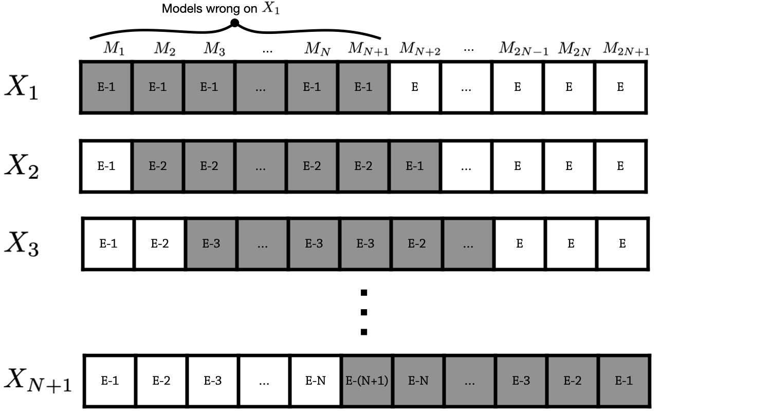
We will prove this by exhibiting a suitable collection of error assignments. Let us start by subtracting $v_1=(1,\dots,1,0,\dots,0)$ with $n+1$ nonzero entries. We then build $v_{i+1}$ from $v_i$ by applying a circular permutation to its entries (i.e. $v_2=(0,1,\dots,1,0,\dots,0)$ and so on).
If we subtract the first vector, the budget will look like $$B_1 = B-v_1 = (E-1,\dots,E-1,E,\dots,E).$$ After one more step, we get $$B_2 = B-v_1-v_2 = (E-1, E-2, \dots, E-2, E-1,\dots,E).$$ After $n+1$ total steps, we get this nice valley pattern: $$B_{n+1} = (E-1,\ E-2,\ E-3,\ \dots,\ E-n,\ E-(n+1),\ E-n,\ \dots,\ E-3,\ E-2,\ E-1),$$ which should be clear because for the first $n$ entries, their position is the number of vectors they get subtracted before the “window of $1$s” leaves them, and the reverse happens for the last $n$ entries. The middle entries is subtracted for every single of these first $n+1$ steps.
The whole procedure is summarized in the figure below:
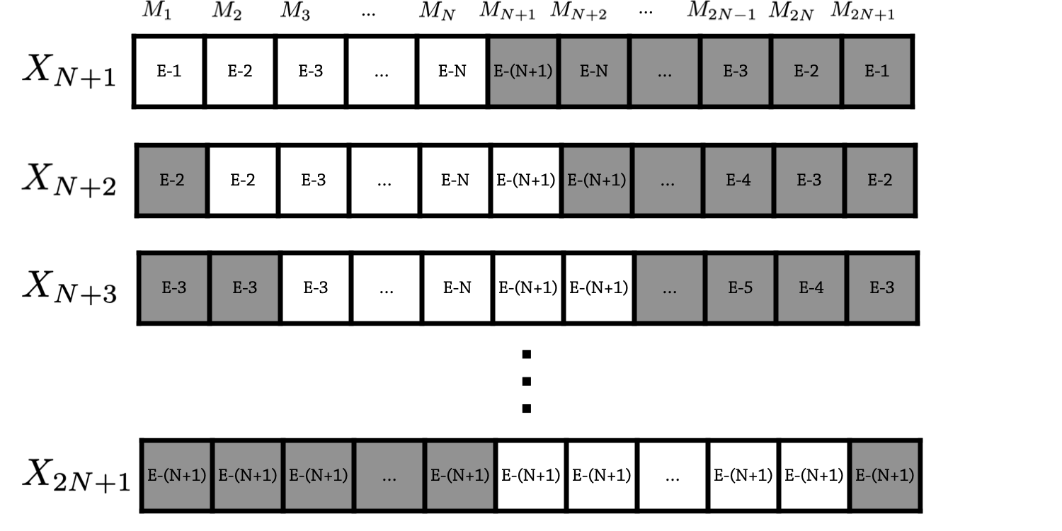
Now if we apply one more step, we see that the window applies to the last $n$ entries and the first one. Going on for a total of $n$ steps, each one of the last $n$ entries will be covered by the window exactly the number of times needed to reach $E-(n+1)$, and the same will happen for the first $n$, while the middle entry will be left untouched.
So after $2n+1$ steps, we reach a symmetric situation gain with
$$B_{2n+1}=(E-(n+1),\dots,E-(n+1)),$$
as illustrated below
Which means that if $E=p(n+1)$, we can repeat these $2n+1$ steps $p$ times, and thus that we did a total of $p(2n+1)$ steps, which is the number of mistakes our ensemble made.
Why is this the worst-case scenario? After these $p(2n+1)$ steps, the error budget of all models is completely exhausted since $$B_{p(2n+1)} = (0,\dots 0).$$
Putting it all together
For any error budget $E$, we have the framing inequality
$$(n+1)\left(1+\left\lfloor\frac{E}{n+1}\right\rfloor\right) \geq E\geq (n+1)\left\lfloor\frac{E}{n+1}\right\rfloor.$$
(Which is just the statement that $E$ is framed bt two multiples of $n+1$)
For the two values framing $E$, we have an exact value for $E^*_\text{ens}$, because they are of the form $p(n+1)$ with
$$p=1+\left\lfloor\frac{E}{n+1}\right\rfloor\text{ and } p=\left\lfloor\frac{E}{n+1}\right\rfloor\text{ respectively.}$$
Therefore, the desired framing inequality is true: $$ (2n+1) \left(1+\left\lfloor\frac{E}{n+1}\right\rfloor\right) \geq E^*_\text{ens} \geq (2n+1) \left\lfloor\frac{E}{n+1}\right\rfloor.$$